In many laboratory magnet systems, users often request “good field linearity.”
However, in real electromagnet or coil systems, linearity is not an abstract concept. It must be defined through measurable relationships between current and magnetic field.
Understanding magnetic field linearity requires examining the B–I calibration curve, saturation effects in magnetic materials, and the methods used to evaluate deviations from ideal behavior.
This article explains what “field linearity” means in practice and how calibration curves are used to verify it.
Why Magnetic Field Linearity Matters
Many experimental measurements rely on a predictable relationship between electrical current and magnetic field.
Examples include:
- Hall effect measurements
- magnetoresistance studies
- magnetic hysteresis experiments
- sensor calibration
If the magnetic field does not scale predictably with current, measurement accuracy may be affected.
In ideal systems, the magnetic field generated by a coil follows a simple relationship derived from electromagnetic theory.
Background information on magnetic fields produced by currents can be found here:
https://en.wikipedia.org/wiki/Biot%E2%80%93Savart_law
In practice, real magnet systems deviate from this ideal behavior.
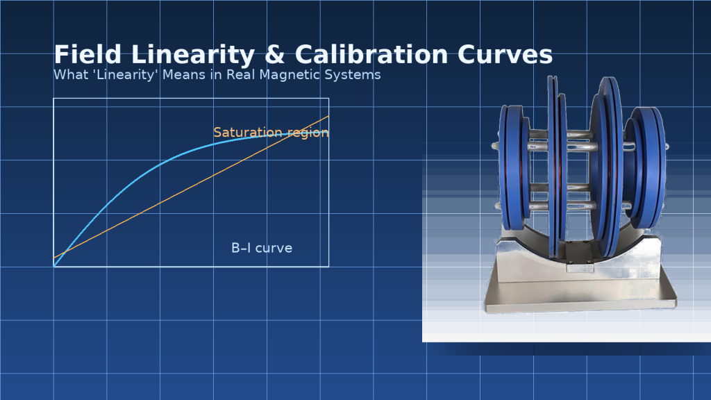
The B–I Curve: Current vs Magnetic Field
The B–I curve describes the relationship between the applied current (I) and the resulting magnetic field (B).
In a perfectly linear system:
B ∝ I
This means that doubling the current doubles the magnetic field.
However, real systems often show deviations due to:
- magnetic core materials
- temperature changes
- coil geometry
- magnetic saturation
Therefore, the actual field must be measured and calibrated.
Magnetic Saturation and Nonlinear Behavior
In electromagnets that use ferromagnetic cores, the magnetic material may eventually approach magnetic saturation.
When saturation occurs, increases in current produce progressively smaller increases in magnetic field.
Background on magnetic saturation:
https://en.wikipedia.org/wiki/Magnetic_saturation
Typical B–I curves show three regions:
- Low current region – nearly linear behavior
- Intermediate region – slight deviation from linearity
- Saturation region – strong nonlinear response
Understanding where saturation begins is essential for defining the usable operating range.
How Linearity Is Actually Evaluated
Field linearity is usually quantified by comparing measured field values to a fitted linear model.
Common evaluation methods include:
Linear Fit
A straight line is fitted to the B–I data.
The deviation between measured and predicted values is then calculated.
Residual Error
Residual error represents the difference between measured values and the fitted linear model.
Residuals are often expressed as:
- percentage of full scale
- absolute field deviation
Example specification:
Linearity error < ±0.5% over operating range
Piecewise Linear Models
In systems with slight nonlinear behavior, calibration curves may use piecewise linear fitting.
This approach divides the current range into smaller segments and fits separate linear models.
This allows accurate field control even when the system is not perfectly linear.
Why Calibration Curves Are Essential
Even well-designed magnet systems require calibration.
Calibration typically involves measuring the magnetic field using a field probe, such as:
- Hall sensors
- fluxgate magnetometers
- NMR probes
Measured values are then used to generate a calibration curve that relates current to field.
This curve allows experimental software to convert desired field values into the correct drive current.
Calibration ensures that the magnet system delivers predictable and repeatable field values.
Practical Linearity Expectations in Electromagnet Systems
In most laboratory electromagnets and coil systems, perfect linearity is not required.
Instead, researchers typically define an acceptable linear operating region.
Typical practices include:
- operating below saturation limits
- using calibrated B–I curves
- applying software compensation
These methods allow high measurement accuracy even when the system is not mathematically perfect.
Linearity and System-Level Magnet Design
Magnetic field linearity depends on several system components:
- coil geometry
- magnetic circuit design
- current source stability
- temperature stability
Cryomagtech provides electromagnet and Helmholtz coil systems designed for stable and predictable magnetic field generation, supporting accurate calibration and repeatable measurements.
👉 Product Link Placeholder – Electromagnet and Helmholtz Coil Systems
Reliable magnet design ensures that calibration curves remain stable over time and across operating conditions.
Key Takeaways
- Magnetic field linearity refers to the relationship between current and magnetic field
- Real magnet systems exhibit nonlinear behavior due to saturation and geometry
- B–I calibration curves are used to quantify system performance
- Residual error and linear fits define usable operating ranges
- Calibration ensures predictable field control in laboratory experiments
Understanding field linearity helps researchers interpret magnetic measurements with confidence.