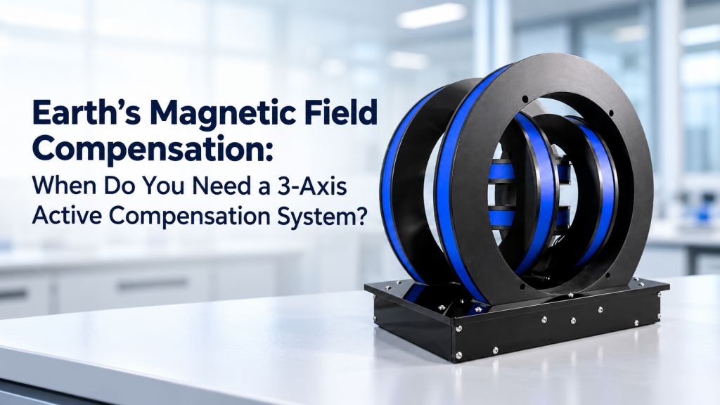
Earth magnetic field compensation using a 3-axis Helmholtz coil and active field control system

The Earth’s magnetic field is weak compared with the fields produced by many laboratory electromagnets.

But for magnetometers, IMUs, electronic compasses, aerospace sensors, low-field magnetic experiments, and precision calibration systems, it can be one of the largest background signals in the room.

A common requirement therefore appears in magnetic field system RFQs:

“We need to compensate the Earth’s magnetic field.”

The next question should be:

Do you need to compensate one field component—or the complete three-dimensional magnetic field vector?

That distinction determines whether a simple single-axis coil is sufficient or whether the application genuinely requires a 3-axis active magnetic field compensation system consisting of:

Three orthogonal coil pairs
Three independent power channels
Magnetic field measurement
Feedback control
Coordinate definition
Field calibration
Compensation software

The objective is not always to create “zero magnetic field.”

Sometimes the real requirement is to reduce one environmental component.

Sometimes it is to create a controlled geomagnetic vector.

And sometimes the experiment genuinely requires the total residual field to approach zero in all three dimensions.

This guide explains how to tell the difference.

1. Earth’s Magnetic Field Is a Vector, Not a Single Number

A useful starting point is understanding what must actually be cancelled.

NOAA describes the Earth’s magnetic field using several quantities, including:

X — northward field component
Y — eastward field component
Z — vertical field component
H — horizontal intensity
F — total magnetic field intensity
D — declination
I — inclination

The total field intensity at the Earth’s surface is typically about 25,000–65,000 nT, equivalent to approximately 25–65 µT or 0.25–0.65 G, depending on location. NCEI

The important point is:

The Earth’s field has both magnitude and direction.

It can therefore be represented as:

Bambient = [Bx, By, Bz]

That is why complete geomagnetic compensation is naturally a three-axis problem.

NOAA NCEI — Geomagnetism Frequently Asked Questions

2. What Does “Earth-Field Compensation” Actually Mean?

This phrase can describe several very different objectives.

Objective A — Cancel one field component

For example:

Reduce the vertical Z field at the sample position.

This may require only one coil axis.

Objective B — Reduce the total background field

For example:

Reduce the three-dimensional ambient field around a magnetometer from approximately 50 µT to below 1 µT.

Now all three components matter.

Objective C — Generate a defined field after compensation

For example:

Cancel the local Earth field, then generate [30, −10, 40] µT for sensor testing.

Now the system must perform both:

Compensation
Controlled vector field generation

Objective D — Maintain a near-zero field despite environmental changes

Now the system needs active feedback.

These are four different system architectures.

A quotation should not begin until the objective is clear.

3. When One-Axis Compensation Is Enough

Not every project needs three axes.

A single-axis coil may be sufficient if:

The experiment is sensitive to only one magnetic direction
The DUT has one relevant sensing axis
Only one environmental component causes measurement error
Mechanical orientation is fixed
Total vector field does not need to approach zero

Example

Suppose a measurement system is sensitive only to vertical field Z.

Ambient conditions are:

Bx = +20 µT
By = −5 µT
Bz = +42 µT

If X and Y have no effect on the measurement, a Z-axis compensation coil can generate approximately:

Bz,coil ≈ −42 µT

and greatly reduce the relevant disturbance.

There is no engineering benefit in adding two unused axes simply because the Earth’s magnetic field is three-dimensional.

4. When You Really Need Three-Axis Compensation

Three-axis compensation becomes appropriate when the total magnetic vector matters.

Typical applications include:

3-axis magnetometer calibration
IMU testing
Electronic compass testing
Aerospace attitude sensors
Navigation systems
Low-field Hall or magnetoresistive sensors
Precision magnetic experiments
Near-zero-field instrumentation
Vector magnetic field simulation

In these applications, suppressing only X while leaving Y and Z unchanged is not sufficient.

The compensation objective becomes

If:

Bambient = [Bx,a, By,a, Bz,a]

then ideally:

Bcoil ≈ [−Bx,a, −By,a, −Bz,a]

so that:

Btotal = Bambient + Bcoil ≈ [0,0,0]

That is the basic logic of 3-axis active compensation.

5. The Word “Zero” Needs a Numerical Definition

“Zero magnetic field” is not an engineering specification.

A buyer should define the allowable residual field.

For example:

<10 µT
<1 µT
<100 nT
<10 nT
<1 nT

These requirements belong to very different technical categories.

Going from 50 µT to 5 µT

is very different from:

Going from 50 µT to 5 nT

The second requirement is 10,000 times smaller.

That affects:

Sensor selection
Current-source resolution
Electrical noise
Environmental control
Mechanical construction
Feedback strategy
Magnetic materials
System location

So always define the target residual field numerically.

6. A Conventional Hall Gaussmeter Is Not Always the Right Feedback Sensor

This is an important purchasing point.

A complete magnetic field system may include a gaussmeter.

But for very low residual-field compensation, buyers should confirm whether the instrument has sufficient:

Resolution
Noise performance
Zero stability
Accuracy

A conventional Hall probe that performs well at millitesla or tesla levels may not be ideal when the target residual field is in the nanotesla range.

Depending on the application, feedback sensing may instead use:

Fluxgate magnetometer
High-sensitivity vector magnetometer
Optically pumped magnetometer
Specialized low-field magnetic sensor

For moderate Earth-field measurement and calibration, an appropriate high-resolution gaussmeter may be sufficient.

The sensor should be selected from the required residual field, not from the assumption that every magnetic field system needs the same probe.

7. What Makes a Compensation System “Active”?

A coil alone is not necessarily an active compensation system.

Open-loop compensation

The system first measures the ambient field.

Then it calculates the required opposite coil field.

For example:

Ambient:

Bx = +28 µT

Coil constant:

Kx = 100 µT/A

Required current:

Ix ≈ −0.28 A

The system sets that current and leaves it there.

This is open-loop compensation.

Closed-loop active compensation

A sensor continuously measures the residual field.

The controller continuously adjusts coil current.

The control architecture becomes:

Environmental Field

↓

Field Sensor

↓

Controller

↓

Bipolar Power Supply

↓

Compensation Coil

↓

Corrected Field

↓

Sensor Feedback

That feedback loop is what makes the system truly active.

8. Open-Loop Compensation Can Be Enough in a Stable Laboratory

Closed-loop control is not always necessary.

If:

Ambient field is stable
Nearby equipment does not change
Required residual field is moderate
Measurements are short
Coil current is highly stable

then the laboratory may:

Measure Bx / By / Bz
Calculate compensation currents
Apply them
Periodically verify the result

For many sensor calibration applications, this is simpler and perfectly practical.

Do not add a complex feedback architecture unless the experiment actually benefits from it.

9. Active Feedback Matters When the Environment Changes

The problem changes when external magnetic disturbances are dynamic.

Possible disturbance sources include:

Elevators
Vehicles
Laboratory machinery
Nearby electromagnets
Motors
Moving ferromagnetic objects
Power cables
Building infrastructure
Operator movement
Equipment switched on or off

NOAA also notes that the measured geomagnetic field contains contributions from several sources and changes with both location and time. NCEI

If those variations are comparable to the allowable residual field, a fixed compensation current may not be enough.

Now active feedback becomes useful.

10. Three-Axis Feedback Means Three Independent Correction Channels

For a 3-axis system:

Bx,error = Bx,target − Bx,measured

By,error = By,target − By,measured

Bz,error = Bz,target − Bz,measured

The controller uses these errors to adjust:

Each coil axis therefore needs its own calibrated relationship between current and magnetic field.

Conceptually:

Bx = KxIx

By = KyIy

Bz = KzIz

where Kx, Ky, and Kz are the axis-specific coil constants.

11. A 3-Axis Helmholtz Coil Is a Natural Architecture for Small-Volume Compensation

A three-axis Helmholtz coil system places three approximately orthogonal coil pairs around the experimental region.

Each pair controls one magnetic field component.

This architecture offers:

Open access to the DUT
Independent X/Y/Z control
Relatively uniform central field
Bipolar compensation
Vector field synthesis
Programmable field sweeps

Cryomagtech’s Helmholtz Coil platform includes 1D, 2D, and 3D configurations and can integrate precision bipolar power supplies, field measurement, and control software for magnetic field simulation, calibration, and external field compensation. Cryomagtech

👉 Product link placeholder: Cryomagtech 3-Axis Helmholtz Coil Active Magnetic Field Compensation System

Suggested internal page:

Cryomagtech Helmholtz Coil Systems for Magnetic Field Compensation

12. Active Compensation Does Not Mean the Whole Room Is Compensated

This is a very common misunderstanding.

A 3-axis Helmholtz coil may produce an excellent compensated field near its center.

That does not mean:

the entire room is near zero field.

Every coil system has a finite useful volume.

The compensation requirement should therefore define:

Required residual field
Required uniformity
Required compensated volume

For example:

Residual field ≤1 µT within a 100 × 100 × 100 mm³ region

is meaningful.

Simply writing:

“Earth magnetic field cancellation required”

is not.

13. The Larger the Compensation Volume, the Harder the Project Becomes

Suppose two laboratories both require:

Residual field ≤1 µT

Laboratory A

Working volume:

100 × 100 × 100 mm

Laboratory B

Working volume:

1 × 1 × 1 m

These are very different systems.

The larger system may require:

Larger coils
More structural support
More copper
More power
More field mapping
Better environmental modeling

At some scale, simple benchtop Helmholtz geometry may no longer be the best architecture.

Room-scale rectangular, biplanar, or customized compensation coils may become more appropriate.

14. A Larger Coil Does Not Automatically Mean Better Compensation

Larger coils can enlarge the useful field region.

But they also introduce trade-offs.

For an ideal Helmholtz coil:

B ∝ NI/R

So as radius R increases, maintaining the same field requires more ampere-turns.

That can mean:

More turns
More current
More electrical power
More heat
Larger power supplies

Earth-field compensation itself requires only tens of microtesla in many cases, so field magnitude is usually modest.

But very large compensation volumes can still create substantial mechanical and electrical systems.

15. Three-Axis Compensation Is About Direction as Much as Magnitude

Suppose the total ambient field magnitude is:

50 µT

A buyer might say:

“So we need a 50 µT compensation coil.”

That is incomplete.

Imagine:

Bambient = [20, 10, 44.7] µT

The magnitude is approximately 50 µT.

But the compensation system needs the correct field on each axis.

Applying −50 µT along X would not cancel the field.

It would create another vector.

The direction matters.

16. Compensation and Geomagnetic Simulation Use the Same Hardware Differently

This is one of the advantages of a programmable 3-axis Helmholtz Coil System.

Suppose the ambient field is:

Bambient = [25, −5, 40] µT

To create approximately zero field

Command:

Bcoil ≈ [−25, +5, −40] µT

To simulate a desired target field

Suppose:

Btarget = [30, 10, 20] µT

Then conceptually:

Bcoil = Btarget − Bambient

So:

Bcoil ≈ [5, 15, −20] µT

The system is no longer simply “cancelling Earth.”

It is creating a controlled net magnetic environment.

That is extremely useful for magnetometer and navigation sensor testing.

17. This Matters for IMU and Electronic Compass Testing

Electronic compasses and magnetic heading systems operate relative to the Earth’s magnetic field.

Their output can depend on:

Heading
Inclination
Sensor orientation
Hard-iron offsets
Soft-iron distortion
Axis calibration

A three-axis coil system can keep the DUT mechanically stationary while electronically changing the surrounding magnetic vector.

That can simplify:

Heading simulation
Orientation sweeps
Vector calibration
Repeatability testing
Automated production tests

The same system can first compensate the laboratory background field and then generate the desired test vector.

18. Aerospace Testing Is Also Naturally Vector-Based

Many aerospace magnetic sensors need to operate in a known vector magnetic environment.

Applications may include:

Satellite attitude determination
UAV navigation
Aircraft magnetic sensors
Spaceborne magnetometers
Magnetic torquer testing
Navigation subsystem validation

A single-axis compensation coil cannot reproduce arbitrary three-dimensional field orientations.

Three independent magnetic axes are usually much more useful when the test requirement involves:

field direction + magnitude + orientation.

19. Scientific Research Shows Why Three-Dimensional Compensation Matters

A Scientific Reports study on a vector magnetometer for space applications used three sets of Helmholtz coils, one for each spatial dimension, driven independently to provide magnetic field cancellation. The architecture maintained a low-field region around the sensor while measuring the components being cancelled. Nature

This is a useful example of the underlying principle:

If the sensor responds to three-dimensional magnetic fields, full vector cancellation requires independent control in three dimensions.

Scientific Reports — Vectorized Magnetometer for Space Applications

20. Very Sensitive Magnetometers Raise the Difficulty Dramatically

For some high-sensitivity instruments, Earth-field compensation is only the first stage.

Optically pumped magnetometers, for example, can require extremely low background fields.

Scientific Reports research on magnetoencephalography notes that some highly sensitive OPMs have operating ranges of only approximately ±5 nT, requiring strong suppression of background field and active compensation of residual fields. Nature

Compare:

Earth field ≈ tens of µT

with:

allowable sensor field ≈ a few nT

That can require suppression by several orders of magnitude.

At that point the project is no longer a simple “3-axis Helmholtz coil” purchase.

It may require:

Magnetic shielding
Active compensation coils
Gradient compensation
Ultra-low-noise current sources
High-sensitivity sensors
Careful material selection

Scientific Reports — Magnetic Field Compensation Coil Design for Magnetoencephalography

21. Active Compensation Is Not the Same as Magnetic Shielding

These terms are often confused.

Passive magnetic shielding

Typically uses high-permeability materials to redirect magnetic flux around the protected volume.

Advantages can include:

No feedback electronics
No continuous control current
Suppression of external disturbances

But shielding can be:

Heavy
Expensive
Mechanically restrictive
Difficult for large open-access systems

Active magnetic compensation

Measures or estimates external field and generates an opposing field using coils.

Advantages include:

Open access
Programmable correction
Adjustable field target
Dynamic compensation

But it requires:

Sensors
Electronics
Calibration
Limited compensated volume

For very demanding applications, passive shielding and active compensation may be combined.

22. Uniform Field Compensation Does Not Automatically Cancel Field Gradients

This is another critical limitation.

A standard 3-axis Helmholtz system is primarily designed to generate relatively uniform magnetic fields.

Suppose the ambient field across a large volume is:

At one side:

Bx = 20 µT

At the other side:

Bx = 28 µT

A uniform compensation field of:

−24 µT

might reduce the average field.

But residual spatial variation remains.

This is a field gradient problem.

23. When Do You Need Gradient Compensation?

Gradient compensation becomes important when:

The compensated volume is large
The experiment is highly sensitive
Nearby magnetic structures distort the field
Sensors move through the working volume
Multiple sensors occupy different positions

A more advanced compensation system may therefore control not only:

but also spatial gradients such as:

dBx/dx
dBx/dy
dBy/dz
etc.

Scientific Reports research on compensation coils shows how separately controlled coil structures can generate both uniform fields and field gradients for advanced magnetic compensation applications. Nature

This is beyond what a basic three-axis Helmholtz system is intended to solve.

24. Place the Feedback Sensor Where It Represents the Experiment

Sensor placement is one of the most important system-design decisions.

Imagine the DUT sits at the center.

The feedback magnetometer sits:

300 mm away.

The controller perfectly drives the field to zero at the feedback sensor.

Does that mean the DUT sees zero field?

Not necessarily.

If spatial gradients exist, the field may be different at the two positions.

Ideally, the feedback sensor should:

Represent the DUT location
Remain within the calibrated uniform region
Avoid disturbing the DUT
Avoid magnetic contamination
Have known XYZ orientation

This becomes particularly important for tight residual-field requirements.

25. But the Probe and the DUT Cannot Always Occupy the Same Position

This creates a practical design problem.

Possible solutions include:

Reference sensor beside the DUT

Measure nearby field and establish the relationship to the true DUT position.

Removable calibration sensor

Measure the field at the DUT position before installing the DUT.

Multiple reference sensors

Use several sensors to estimate the field over a larger region.

DUT sensor as feedback

In some specialized applications, the DUT itself provides magnetic field information.

Each option has trade-offs.

The correct method depends on required accuracy and experimental geometry.

26. Sensor Orientation Must Match the Coil Coordinate System

For three-axis compensation, the controller must know how sensor coordinates relate to coil coordinates.

Suppose the sensor reports:

but the coil system uses:

If the sensor is rotated relative to the coil frame, the components cannot simply be copied directly.

A coordinate transformation may be required.

This is why a serious 3-axis compensation system should document:

+X direction
+Y direction
+Z direction
Sensor orientation
Coil orientation
Origin
Right-handed coordinate convention

Otherwise the controller may compensate the wrong direction.

27. Cross-Axis Coupling Should Be Calibrated

An ideal X coil would generate only Bx.

A real coil system may generate small unwanted Y and Z components because of:

Mechanical misalignment
Manufacturing tolerances
Nearby magnetic materials
Non-orthogonal axes

The real system may therefore be represented more accurately by a matrix:

B = M · I + Bambient

where:

B is the measured field vector
I is the three-axis current vector
M is the calibrated coil-response matrix

For higher-precision compensation, software can use the inverse relationship to calculate the required currents.

That is more accurate than assuming three perfectly independent scalar coil constants.

28. The Compensation Range Should Exceed the Expected Ambient Field

If the local Earth’s field is approximately 50 µT, designing the system for exactly ±50 µT per axis leaves little margin.

Additional field may be required for:

Local building fields
Magnetic equipment
Sensor offset
Future test vectors
Environmental variation

For many Earth-field applications, reasonable engineering headroom is useful.

But the same principle applies as with all magnetic systems:

Do not overspecify without a reason.

A sensor requiring ±100 µT environmental simulation does not automatically benefit from a ±50 mT coil.

29. Compensation Resolution Can Matter More Than Maximum Field

Suppose your application needs to reduce the field to:

<100 nT

A system capable of ±10 mT but adjustable only in coarse steps may be less useful than a ±200 µT system with excellent:

Current resolution
Noise
Stability
Zero repeatability

For low-field compensation, buyers should evaluate:

Maximum field
Minimum field increment
Noise
Drift
Current stability
Sensor noise
Residual field

not just maximum magnetic field.

30. Current-Source Noise Directly Becomes Magnetic-Field Noise

If:

B = K × I

then current variation produces field variation:

ΔB = K × ΔI

That means a noisy power supply creates a noisy compensated magnetic environment.

For precision low-field work, a high current rating alone is not enough.

Important characteristics include:

Current resolution
Short-term noise
Long-term stability
Zero-crossing behavior
Bipolar performance

This is one reason low-field magnetic systems require different design priorities from high-field electromagnets.

31. Temperature Drift Can Also Affect Compensation

As coils heat:

Copper resistance changes
Mechanical dimensions may shift
Electronics can drift

If current regulation is excellent, resistance change may not directly change field much in a simple air-core coil.

But thermal effects can still affect:

System stability
Sensor zero
Mechanical geometry
Long-duration calibration

For demanding compensation systems, temperature should therefore be considered in the stability budget.

32. Dynamic Compensation Needs a Defined Bandwidth

A buyer may request:

“Automatic environmental field compensation.”

The missing question is:

How fast must the system respond?

Examples:

Slow compensation

Correct changes over:

Minutes
Hours

Useful for:

Thermal drift
Slow ambient changes

Faster compensation

Correct changes at:

1 Hz
10 Hz
Higher frequencies

Now coil inductance, controller bandwidth, sensor bandwidth, power-supply response, and control-loop stability become increasingly important.

A system designed for static Earth-field cancellation should not automatically be assumed to cancel fast magnetic disturbances.

33. Feedback Bandwidth Should Match the Disturbance Spectrum

There is little benefit in building a 1 kHz compensation loop if relevant environmental variation occurs only over minutes.

Likewise, a very slow loop cannot suppress rapid disturbances from:

Moving machinery
Electrical switching
Nearby magnetic actuators

A good specification should therefore describe:

Static residual target
Relevant disturbance frequencies
Required compensation bandwidth

This allows the control system to be designed rationally.

34. Avoid Feedback Instability

Three-axis closed-loop compensation is a control problem.

If loop gain is too aggressive, the system may:

Oscillate
Overshoot
Inject magnetic noise

If it is too slow, compensation may lag behind the disturbance.

A robust controller should account for:

Sensor dynamics
Coil inductance
Power supply response
Sampling rate
Axis coupling
Filtering

More feedback is not automatically better.

Stable feedback is better.

35. Nearby Magnetic Materials Can Defeat an Otherwise Good System

A 3-axis compensation coil may be designed correctly and still perform poorly after installation.

Common problems include:

Steel optical tables
Ferromagnetic screws
Motors
Loudspeakers
Equipment racks
Reinforced concrete
Magnetic tools

These objects may create:

Static offsets
Field gradients
Local distortion

For low-residual-field applications, installation environment matters almost as much as coil performance.

36. “Compensated Volume” Should Be Defined Like Any Other Uniform-Field Volume

A useful requirement may say:

Residual vector field ≤1 µT within a 200 × 200 × 200 mm³ central volume.

A more demanding specification might say:

Residual field magnitude ≤100 nT within a 100 mm diameter spherical volume.

Now the supplier knows both:

Required suppression
Required spatial region

Without the volume, the residual-field number is incomplete.

37. Factory Compensation Performance May Differ from On-Site Performance

The supplier can characterize:

Coil constants
Axis alignment
Uniformity
Control accuracy

at the factory.

But the customer’s site has its own magnetic environment.

Therefore Earth-field compensation often requires on-site steps such as:

Install the system
Measure local Bx / By / Bz
Check magnetic gradients
Determine compensation currents
Tune feedback
Verify residual field

This is particularly important when surrounding structures are unknown.

38. One-Time Background Measurement May Not Be Enough

Suppose the field is measured Monday morning:

[25, −4, 42] µT

and compensation is configured.

Later:

An elevator begins operating
A large instrument turns on
A steel cart moves nearby

Now the background changes.

For applications requiring only several microtesla accuracy, that may not matter.

For sub-microtesla or nanotesla requirements, it can matter greatly.

That is the practical threshold where continuous field monitoring becomes increasingly valuable.

39. A Practical 1-Axis Example

Application:

Single-axis magnetic sensor
Z-axis sensitivity only
Ambient Z ≈ 40 µT
Required residual Z <5 µT
X/Y field irrelevant

Recommended architecture:

1-axis Helmholtz coil
Bipolar current source
Single-axis field measurement
Open-loop or simple feedback

A three-axis system would likely be unnecessary.

40. A Practical 3-Axis Magnetometer Calibration Example

Application:

3-axis magnetometer
Ambient field ≈50 µT
Target test range ±100 µT
DUT fixed in position
Vector calibration required

Recommended architecture:

3-axis Helmholtz coil
Three bipolar power channels
Vector field measurement
PC control
Background compensation
Programmable XYZ field synthesis

Now three axes provide direct experimental value.

41. A Practical Aerospace Sensor Test Example

Application:

Navigation sensor
Earth-field simulation
Adjustable heading and inclination
Fixed DUT
Automated test sequence

The system needs to produce arbitrary field vectors.

Recommended architecture:

3-axis Helmholtz Coil + vector control + background compensation

The workflow becomes:

Measure ambient field
Subtract it from desired target vector
Calculate XYZ currents
Generate corrected field
Verify with reference sensor

This is much more than simple field cancellation.

42. A Practical Near-Zero-Field Research Example

Application:

Highly sensitive magnetometer
Required residual field in nT range
Large experimental volume
Significant room gradients

A basic 3-axis Helmholtz system may no longer be enough.

The project may require:

Magnetic shielding
Customized active coils
Gradient coils
Multiple high-sensitivity sensors
Advanced feedback

This is where buyers should stop asking:

“What size Helmholtz coil do we need?”

and start treating the problem as:

magnetic environment engineering.

43. What Information Should Be in an RFQ?

For an Earth-field compensation project, provide:

Application

What is being measured or calibrated?

DUT

Dimensions
Sensitive volume
Can it move or rotate?

Ambient Field

If known:

Required Residual Field

For example:

≤1 µT resultant

Compensation Volume

For example:

300 × 300 × 300 mm³

Number of Axes

Dynamic Requirement

Static
Slow drift compensation
Required bandwidth

Measurement

Gaussmeter
Fluxgate
Other reference magnetometer

Control

Open-loop
Closed-loop
PC control
Ethernet / USB if required

This information makes system selection much more accurate.

44. Seven Questions That Determine Whether You Really Need Three Axes

1. Does the total vector field matter?

If yes, three axes are usually appropriate.

2. Is the DUT sensitive in X, Y, and Z?

If yes, consider three-axis compensation.

3. Must the residual total field approach zero?

If yes, all three ambient components matter.

4. Will you simulate arbitrary geomagnetic vectors?

If yes, three axes are strongly justified.

5. Can the DUT simply be rotated?

For some calibration tasks, mechanical rotation may reduce required magnetic axes.

6. Is the environment changing during the experiment?

If yes, active feedback may be required.

7. Is the requirement actually a gradient problem?

If yes, three uniform-field axes alone may not solve it.

These questions are more useful than simply asking:

“Do you want a 3-axis system?”

45. Open-Loop vs. Closed-Loop Selection

A simple rule is:

Use open-loop when:

Ambient field is reasonably stable
Residual-field tolerance is moderate
Periodic calibration is acceptable
Simplicity matters

Consider closed-loop when:

Ambient field changes over time
Residual tolerance is tight
External magnetic disturbances are unavoidable
Long-duration stability matters
Automatic compensation is required

Closed-loop control is not inherently superior.

It is appropriate when the disturbance requires feedback.

46. Gaussmeter + Control System: Where It Fits

For suitable field ranges, an integrated system can use:

3-axis Helmholtz coil
Bipolar excitation power supplies
Magnetic field measurement
PC control software
Feedback algorithm

Cryomagtech’s magnetic field generation platform includes systems combining Helmholtz coils, programmable field measurement, power supplies, and PC software. Cryomagtech

For very low residual-field targets, however, sensor selection should be reviewed separately rather than assuming a standard Hall gaussmeter will always provide enough low-field performance.

That distinction helps prevent a system from being electrically powerful but metrologically blind at the field level that actually matters.

47. How Cryomagtech Approaches Earth-Field Compensation Projects

Cryomagtech Magnet & Field Systems can be configured around:

1D / 2D / 3D Helmholtz coils
Precision bipolar current sources
Magnetic field measurement
Open-loop control
Closed-loop field stabilization
XYZ vector field synthesis
Background field compensation
Field mapping
Customized coil dimensions

The correct architecture depends primarily on:

Required residual field
Compensation volume
Environmental stability
Number of controlled axes
Feedback bandwidth
DUT geometry

👉 Product link placeholder: Cryomagtech 3-Axis Helmholtz Coil + Gaussmeter + Active Magnetic Field Compensation System

Suggested internal page:

Cryomagtech Magnetic Field Generation Systems

The most useful inquiry is therefore not:

“Please quote a system to cancel the Earth’s magnetic field.”

It is:

“We need to reduce the ambient XYZ magnetic field to below 1 µT within a 300 × 300 × 300 mm³ volume, with continuous monitoring and automatic compensation.”

That is an engineering specification.

48. Key Takeaways

When specifying Earth’s magnetic field compensation, remember:

The Earth’s magnetic field is a three-dimensional vector.
Surface field magnitude is typically around 25–65 µT, depending on location. NCEI
One-axis compensation is enough when only one field component affects the experiment.
Three-axis compensation is appropriate when the total vector field matters.
A 3-axis system can both cancel ambient field and generate controlled target vectors.
“Zero field” must always be given a numerical residual-field target.
1 µT and 1 nT requirements represent very different engineering challenges.
Open-loop cancellation can be sufficient in a stable laboratory.
Active closed-loop compensation becomes valuable when the environment changes.
A feedback sensor must have enough resolution and stability for the residual-field target.
A standard Hall gaussmeter is not automatically suitable for ultra-low-field compensation.
Feedback sensor position and orientation matter.
Cross-axis coupling should be calibrated for precision vector control.
The compensated volume must be specified together with residual field.
A 3-axis Helmholtz system primarily cancels uniform field components; gradients may require additional coil architecture.
Large-volume near-zero-field projects may require magnetic shielding, active coils, and gradient compensation together.
Current-source noise, sensor noise, thermal drift, and feedback bandwidth all become important as the residual-field target becomes smaller.
Factory coil performance does not remove the need to characterize the customer’s actual magnetic environment.

The central decision is therefore simple:

If your experiment only cares about one magnetic direction, do not automatically buy three-axis compensation.

But if you need to control the complete magnetic vector—especially for magnetometers, IMUs, navigation sensors, aerospace testing, or near-zero-field research—then three independent axes become part of the measurement method rather than an optional upgrade.

References

1. NOAA National Centers for Environmental Information — Geomagnetism Frequently Asked Questions

NOAA describes the Earth’s field through X, Y, Z and other geomagnetic components and reports typical total field intensity of approximately 25,000–65,000 nT (25–65 µT). This directly supports the vector-field approach required for full geomagnetic compensation. NCEI

NOAA — Geomagnetism Frequently Asked Questions

2. Scientific Reports — Magnetic Field Compensation Coil Design for Magnetoencephalography

This research demonstrates why highly sensitive magnetic sensors may require active compensation of residual magnetic fields and shows that low-field applications can demand substantially more sophisticated control than simple static Earth-field cancellation. Nature

Scientific Reports — Magnetic Field Compensation Coil Design for Magnetoencephalography