Why Background Magnetic Fields Matter More Than You Think
In an ideal world, every laboratory would have a magnetic shielding room.
In reality, most labs do not.
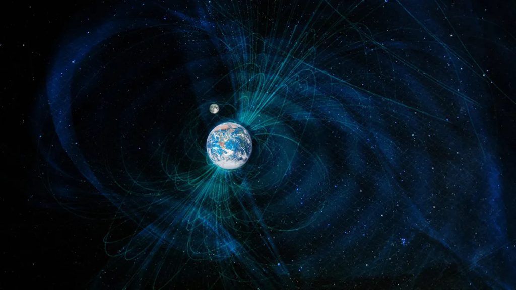
Earth’s magnetic field is typically 25–65 µT, and it is not stable.
Nearby elevators, power lines, vehicles, and even lab equipment cause slow drift and sudden field jumps.
For experiments involving Hall measurements, sensor calibration, AHRS/IMU testing, or low-field material studies, this background field becomes a serious source of error.
This is where background field compensation becomes essential.
When Do You Actually Need Background Field Compensation?
You likely need background field compensation if any of the following apply:
- Your lab does not have a magnetic shielding room
- Your target field is comparable to Earth’s field (µT to low mT range)
- Your experiment runs for hours or overnight
- You require field stability or repeatability, not just peak field strength
- You work with 3-axis sensors such as magnetometers, IMUs, or AHRS modules
In these cases, passive shielding alone is insufficient.
Active compensation becomes the practical solution.
The Basic Principle of Background Field Compensation
Background field compensation works by measuring unwanted magnetic fields and actively canceling them in real time.
The system consists of three core elements:
- Field generation hardware
Typically a 3-axis Helmholtz coil or vector coil system - Magnetic field sensors
Fluxgate, Hall probes, or reference magnetometers - Control software with feedback algorithms
Used to calculate and apply correction currents
The goal is simple:
Make the magnetic field at the sample position equal to the desired setpoint, not the ambient environment.
Sensor Placement: Where Compensation Often Goes Wrong
Sensor placement is one of the most common sources of poor compensation performance.
Recommended practices:
- Place reference sensors as close as possible to the sample volume
- Avoid locations near current-carrying cables or ferromagnetic structures
- Use multi-point sensing for larger uniform volumes
Placing sensors too far from the sample leads to overcompensation or undercompensation, especially in 3-axis systems.
Control Strategies and Compensation Algorithms
Most modern systems use closed-loop field control.
Typical algorithm approaches include:
- PID control for slow drift compensation
- Feedforward + feedback for predictable disturbances
- Low-pass filtering to suppress high-frequency noise
Advanced implementations allow:
- Independent compensation on X, Y, and Z axes
- User-defined stability targets
- Long-term drift monitoring and logging
This is where hardware quality and software design must work together.
Why 3-Axis Systems Are the Preferred Solution
Single-axis compensation can only correct part of the problem.
Earth’s field is vector-based, not scalar.
A 3-axis Helmholtz or vector coil system allows:
- Full vector cancellation of Earth’s magnetic field
- Precise orientation control
- Seamless integration with sensor calibration workflows
👉 Product link placeholder: Cryomagtech 3-Axis Helmholtz / Vector Coil System
Cryomagtech systems combine field generation hardware, precision current drivers, and control software into a unified platform designed for real laboratory conditions.
Reference Sources
For readers who want deeper background, the following references are useful:
- Wikipedia – Earth’s magnetic field
https://en.wikipedia.org/wiki/Earth%27s_magnetic_field - IEEE – Magnetic field compensation and active control methods
https://ieeexplore.ieee.org/
Final Thoughts: Compensation Is Not Optional Anymore
If your experiment depends on accuracy, repeatability, or long-term stability, background field compensation is no longer optional.
With modern 3-axis magnetic field systems and software-based compensation, laboratories can achieve shielding-like performance without building a shielding room.
That is exactly the problem this technology was designed to solve.