Why “Uniformity” Matters More Than a Single Tesla Number
A magnet’s peak field tells only part of the story. For Hall measurements, sensor calibration, materials research, and metrology, magnetic field uniformity often determines whether your data is repeatable, publishable, and comparable across labs.
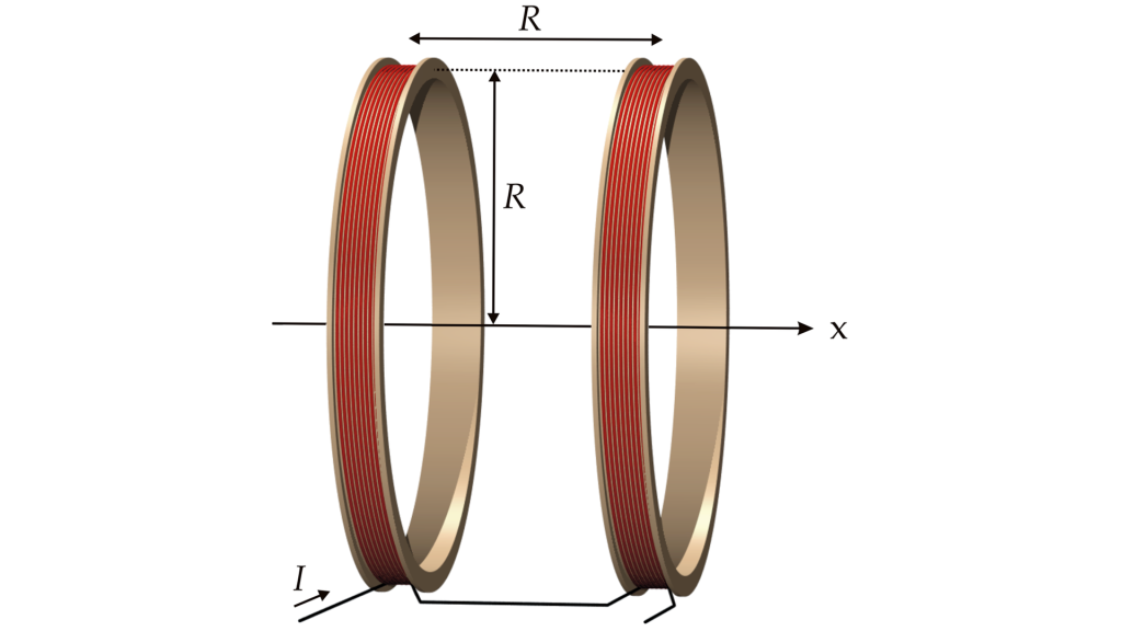
In practice, “uniform” never means perfectly constant everywhere. Instead, uniformity is a measurable tolerance over a defined volume. Helmholtz coils are widely used because they create a region of nearly uniform magnetic field around the center. Wikipedia
1) Define the Uniform Region First
Before you talk about uniformity numbers, define the uniformity region. Buyers often skip this step and end up comparing specs that are not comparable.
Common ways to define the region:
A. Uniform Volume (most common in lab magnets and coils)
- Example: a 50 mm × 50 mm × 50 mm cube
- Or: a cylinder (diameter × length)
B. DSV (Diameter of Spherical Volume)
This is popular in MRI-style homogeneity specs and is useful if your “device under test” is roughly spherical or rotates. Questions and Answers in MRI
C. “Usable Zone” with fixture included (best for procurement)
Define the region after including your sample holder, probe station, or calibration jig.
If your fixture forces the sample off-center, your real uniformity may be worse than the datasheet.
Rule of thumb: the uniformity region should be defined around the actual sample location, not an idealized center point.
2) How Uniformity is Quantified
Uniformity is typically expressed in percent or ppm. The key is to state the formula.
Metric 1: Peak-to-peak uniformity (simple and common)
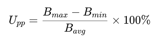
- Easy to measure and communicate
- Great for RFQs and acceptance tests
Metric 2: Deviation from center field (also common)
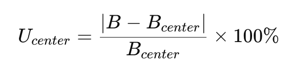
- Useful when the “center” is your reference for calibration
Metric 3: ppm homogeneity (high-end magnets, MRI-style)
- Expresses very small variations over a defined region (often DSV). Questions and Answers in MRI
Important: Always state field level (e.g., at 0.5 T vs 1.0 T). Some systems look “more uniform” at lower fields.
3) How to Measure Magnetic Field Uniformity
Uniformity should be measured with a mapping plan that matches your region definition.
A. Field mapping with a Hall probe (most common)
Best for: Helmholtz coils, electromagnets, vector magnets
Typical setup:
- A calibrated Hall probe (with traceable calibration if possible)
- A 3D positioning stage (manual or motorized)
- A grid or spherical sampling plan
Practical tips:
- Use a stable current source and allow thermal equilibrium before mapping
- Record temperature and time, because drift can fake “non-uniformity”
B. NMR probe (high precision for strong fields)
Best for: high-field superconducting magnets and metrology-level mapping
NMR can offer excellent accuracy, which is why it is commonly referenced in precision magnet field measurements. CERN Document Server
C. Fluxgate / magnetometer arrays (good for low fields)
Best for: Earth-field compensation, µT-level Helmholtz systems, sensor calibration rigs
Works well in the ±100–500 µT range, especially for orientation and bias field control.
4) What Acceptance Criteria Should Look Like
A good acceptance spec is measurable, testable, and leaves no room for interpretation.
Example acceptance statement (copyable)
- Field: 1.000 T
- Uniform region: 20 mm diameter spherical volume (DSV) centered on sample position
- Uniformity metric: peak-to-peak
- Requirement: Upp≤0.10%
- Measurement method: Hall probe mapping, 5×5×5 grid, calibrated probe, report includes raw map and summary table
If you want procurement to go smoothly, specify:
- Region geometry + size
- Field setpoint(s)
- Uniformity formula
- Measurement plan (grid density, probe type)
- Acceptance deliverables (plots + table + calibration certificate)
5) Examples: How to Specify Uniformity for Different Systems
Below are examples (not universal defaults) to show how a “good RFQ spec” looks.
Example A: Helmholtz coil for sensor calibration (µT–mT range)
- Field range: ±300 µT per axis
- Uniform region: 100 mm cube (with fixture installed)
- Uniformity requirement: Upp≤0.5% at ±300 µT
- Stability: ≤0.1%/hour at fixed setpoint
- Notes: include background field compensation if needed
Example B: Electromagnet for Hall measurements (0.1–1 T)
- Field range: 0–1.0 T
- Gap: 40 mm
- Uniform region: 10 mm DSV at sample plane
- Uniformity requirement: Upp≤0.1% at 0.5 T
- Include: field calibration curve vs current; hysteresis handling procedure
Example C: Vector magnet / 3-axis field platform
- Field per axis: specify Bx/By/Bz separately
- Uniform region: define for each axis, because geometry and coupling differ
- Uniformity requirement: stated per axis at defined setpoints
- Coupling spec: cross-axis interference limits (optional but useful)
Where Cryomagtech Fits
If you’re defining uniformity for a new lab setup, the fastest way to avoid mistakes is to start from the real fixture + real sample position, then select the right field source:
- Helmholtz coils: best for calibration, low-field control, and large uniform volumes
- Electromagnets / vector magnets: best for Hall measurements, higher fields, and controlled orientation
👉 Cryomagtech Helmholtz Coil / Vector Magnet Solution
If you share your required uniform volume and field target, Cryomagtech can recommend a practical configuration and an acceptance plan you can actually enforce.
Quick Checklist for Your RFQ (copy-paste)
- Field range and setpoints (e.g., 0.5 T, 1.0 T)
- Uniform region size and geometry (cube/cylinder/DSV)
- Uniformity formula (peak-to-peak or center deviation)
- Probe type and mapping plan (grid density, positioning method)
- Acceptance deliverables (map plot + table + calibration certificate)
References
Magnetic field homogeneity is commonly specified over a defined volume (e.g., DSV), often in ppm. Questions and Answers in MRI
Helmholtz coils produce a region of nearly uniform magnetic field. Wikipedia